A short course on petrophysics

Introduction to log interpretation

Interpretation is defined as the action of explaining the meaning of something. Log Interpretation is the explanation of logs (rb, GR, resistivity etc) in terms of well and reservoir parameters - zones, porosity, and oil saturation.
Logs are employed to give information about the reservoir, from formation tops and marker beds to porosity and permeability of layers, to porosity and fluids and their types.
The data used depends on the needs and the type of wells being evaluated. An exploration well needs more data than a simple development well.
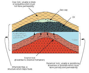
To have a reservoir the elements needed are:

A reservoir rock – stores the hydrocarbon
A source rock (but it may be far away from the actual reservoir) – produces hydrocarbon
The cap rock has to be on top – traps hydrocarbon
The structure must be there – captures fluids

This interpretation of the logs is done by petrophysicists.

Reservoir rocks

The earth is made up of a number of components. At the centre is the solid core which is Nickel - Iron; around this is a liquid core of the same material. The next part is a liquid called the Mantle, composed of much lighter materials. Finally there is a solid crust, a very thin sheath when compared to the total diameter. It is this crust which is of interest to the petroleum engineers as the deepest a well can go remains within this crust.
The crust is not one solid skin on the Mantle. It is broken into a number of irregular “plates “. The plates can be large, the pacific plate, or relatively small, some of the Mediterranean plates. The centers of the plates are stable environments while the edges are the earthquake/volcano regions of the earth. It is these edges in which the petrophysicists are interested. These plates move around driven by the convection currents in the mantle. Two types of features are caused by the movement of these plates. The first set are compressional. Here two plates are pushed together. They can create a zone of mountains or one plate can go under the other creating a “trench”. Mountains are usually associated with trenching as well. On the other side of the currents tensional effects are found. Here the plate is stretched out thin creating faults and rifts and eventually a new plate. Both compressional and tensional features play a large role in the structures of reservoirs.
Going into a greater detail of geography we see that there are primarily three types of rocks:

Igneous rocks – created by volcanoes
Sedimentary rocks – created by the sedimentation of various rocks
Metamorphic rocks – created by the effects of heat and pressure on the above two types

Out of these, the igneous rocks, such as granite, have no porosity or permeability of their own. However, tectonic forces may fracture the rock from these the hydrocarbons can flow to create a reservoir. The metamorphic rocks do not exist in reservoirs. The sedimentary rocks are the most important for the oil industry as they contain most of the source rocks and cap rocks and virtually all reservoirs. Sedimentary rocks can be divided into two types:

Clastic – formed from the materials of the older rocks by the actions of erosion, transportation and deposition. Clastics are mainly sand and shale.
Carbonate – from chemical or biological deposition. Carbonates are clay, limestone, dolomite and anhydrite

The depositional environment affects the grain size. Continental deposits are usually dunes. A shallow marine environment has a lot of turbulence hence varied grain sizes. It can also have carbonate and evaporite information. A deep marine environment produces fine sediments. Note here that fine grains lead to poor permeability.
Rocks are described by three properties:

Rock porosity – quantity of pore space
Rock permeability – ability of a formation to flow
Rock matrix – major constituent of the rock

Precisely defining porosity, it is the fraction of void space occupied by pores or voids. In normal reservoirs it ranges between 20-39%. In a rock the grain size (same size grains) does not affect the porosity. Thus sand, silt and shale can have the same porosity .The differences come in permeability where the grain size has a direct effect, large grains meaning higher permeability. This is the reason that a universal porosity - permeability transform does not work; two rocks with the same porosity but different grain sizes will not have the same permeability. If we look at the clastic and carbonate reservoirs individually we can easily state that in clastic reservoirs:

Porosity is determined mainly by the packing and mixing of grains
Permeability is determined mainly by grain size and packing, connectivity and shale content

In carbonate reservoirs:

Porosity and permeability are determined by the depositional and post-depositional events (such as fracturing)

SP

The SP (Spontaneous Potential) curve is a continuous recording (versus depth) of the difference in potential between a moveable electrode in the borehole and a fixed zero potential surface electrode. Its units are in millivolts. This potential is due to a combination of two phenomena:

electro kinetic potential
In a low permeability formation, where the mudcake is only partially built up, this potential may be as high as 20 mV. This situation is, however, rare and in generalthe total electro kinetic potential can be neglected.
electrochemical potential
This potential is created by the contact of two solutions of different salinity, either by a direct contact or through a semi permeable membrane such as shale.

The total potential drop (which is equal to the Static SP) is divided between the different formations and mud in proportion to the resistances met by the current in each respective medium. The SP, which is the measure of the potential drop in the mud of the borehole, is only part of the SSP. On a log, the SSP is the deflection seen on the SP curve from the shale base line to the sand line.
This curve can be used to distinguish between shale and sand. In saline mud, the SP curve deflects to the positive when moving from shale to sand. On the other hand, in fresh mud it deflects to the negative when moving from shale to sand. A more important use of this log is the determination of the value of Rw. The procedure used for this purpose is:

from the log heading, get Rmf at surface temperature
convert Rmf to formation temperature using chart Gen-9
convert Rmf at formation temperature to Rmfe using:
Rmfe = 0.85 x Rmf for 0.03 Chart SP-2m otherwise
calculate SSP from the log by looking at the maximum deflection in the curve
enter chart SP-1 with SSP and Rmfe to get the Rmfe/Rwe ratio
calculate the value of Rwe from this ratio
enter chart SP-2m with Rwe and formation temperature to get Rw

The charts mentioned in this procedure can be accessed from any log interpretation chart book.
The SP can be affected by a number of surface effects as it relies on the fish as its reference electrode. Power lines, electric trains, electric welding, and radio transmitters create ground currents which disrupt the fish reference, causing a poor, sometimes useless, log.

GR

The gamma ray log is a measurement of the formation’s natural radioactivity. Gamma ray emission is produced by three radioactive series found in the Earth's crust.

Potassium (K40) series
Uranium series
Thorium series

Gamma rays passing through rocks are slowed and absorbed at a rate which depends on the formation density.
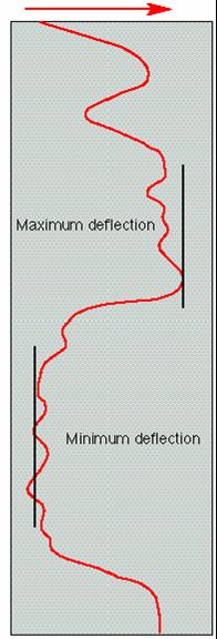
In order to compute the amount of shale from this log, we look at the minimum and the maximum deflections. The minimum value gives the clean 100% shale free zone. The maximum gives the shale zone. All other points can then be calibrated in the amount of shale. Some of the typical values for the gamma ray tools in a variety of formations are:

Limestone <20 API
Dolomite <30 API
Sandstone <30 API
Shale 80-300 API
Salt & anhydrite <10 API

No formation is perfectly clean; hence the GR readings will vary. Limestone is usually cleaner than the other two reservoir rocks and normally has a lower GR.

Neutron porosity

Neutrons start as fast neutrons and rapidly loose energy passing through the epithermal state to reach the thermal range. The process of slowing down is primarily caused by collisions with the hydrogen atoms. The more hydrogen the fewer neutrons reach the detectors.
The final stage is capture by an atom when a capture gamma ray is emitted. The oldest tools measured these gamma rays as there were no reliable neutron detectors at that time. The current neutron tool is the Compensated Neutron Tool (CNT). The CNT measures the neutron population in the thermal region. The count rate for each detector is inversely proportional to porosity with high porosity giving low count rates. The logs have to be corrected for the borehole effects which include the borehole size, the mudcake, the borehole salinity, the mud weight, the temperature and the pressure. Some of the typical values indicated by this tool for various formations are:

Limestone 0
Sandstone -2
Dolomite 1
Anhydrite -2
Salt -3
Shale 30-45
Coal 50+

The primary use of this tool is to measure the porosity. This tool can not only be run in open hole but also in cased hole. However, in the case of cased hole, the corrections required will be different from those of the open hole.
Some elements such as Gadolinium and Boron capture neutrons efficiently. If they are present in the formation, the thermal neutron tools will read a porosity that is too high.

Density

The density tools use a chemical gamma ray source and two or three gamma ray detectors. The number of gamma rays returning to the detector depends on the number of electrons present, the electron density. It is assumed that this electron density is equal to the bulk density of the formation. The LDT tool has two detectors measuring the same density. If there is no mud cake, both will read the same. If there is mud cake there will be a slight difference which can be computed and hence the measurement corrected. The spine and ribs plot is the graphical representation of the method used. In this method, the spine represents the line of increasing formation density on the plot of the long spacing count rate vs. short spacing count rate. The presence of mud cake causes a deviation from the line in a predictable manner. Thus a correction can be made to obtain the true density. The density of each mineral is unique. The tool is calibrated in limestone, sandstone has a lower density and dolomite is higher; shale varies with the precise clay minerals present. The typical values indicated by this tool for various formations are:

Limestone 2.71
Sandstone 2.65
Dolomite 2.85
Anhydrite 2.98
Salt 2.03
Shale 2.2 – 2.7
Coal 1.5

Sonic

The sonic tools create an acoustic signal and measure how long it takes to pass through a rock. By simply measuring this time we get an indication of the formation properties. The amplitude of the signal will also give information about the formation. The travel through the formation is affected by a number of effects, notably the porosity. Hence the tool can be used to measure porosity.
Sonic–BHC is a simple tool that uses a pair of transmitters and four receivers to compensate for caves and sonde tilt. The normal spacing between the transmitters and receivers is 3' - 5'. It produces a compressional slowness by measuring the first arrival transit times.
The BHC tool is affected by near borehole altered zones hence a longer spacing is needed with a larger depth of investigation so long spacing sonic was used instead. The tool spacings are 8' - 10', 10' - 12'. The tool cannot be built with transmitters at each end like a BHC sonde, hence there are two transmitters at the bottom. A system called DDBHC - depth derived borehole compensation, is used to compute the transmit time. The uses of this tool are the same as the BHC tool.
The initial wave from the transmitter is a compressional wave (the particle motion is parallel to the wave motion). It interacts with the surface of the formation mud to create a number of secondary waves. The first of these is the compressional wave in the formation. This is followed by the shear wave (particle motion is perpendicular to wave motion) and finally by the Stoneley wave (the particle motion is elliptical) moving along the interface borehole wall – fluid. All of the waves arriving at the receivers are the head waves generated by the waves in the formation.
In order to extract shear and Stoneley information from the waveform STC processing is used. In this procedure we look for the same part of the wave on each train. Once this has been done the transit time can be computed. The first part of the wave shows coherent signals which are the compressional arrivals, further out are the shear arrivals and finally the Stoneley. The processing looks at all the waveforms together to obtain the final output. If we plot this information on a map, at a given depth the slowness can plotted against time. Regions of large coherence appear as contours.
The first tool to use STC processing was the array sonic which was able to measure shear waves and Stoneley waves in hard formations. However, they were unable to do so in soft formations. So, for this purpose the Dipole Shear Imager (DSI) was developed. The addition in this case is a dipole source. This tool creates a flexural wave on the borehole wall and shear and compressional in the formation. The shear wave is recorded whatever the formation is. Typical sonic readings for various formations are:

Limestone 47.5
Sandstone 51 – 55
Dolomite 43.5
Anhydrite 50
Salt 67
Shale >90
Coal >120
Steel 57

Sonic

Limestone 47.5
Sandstone 51 – 55
Dolomite 43.5
Anhydrite 50
Salt 67
Shale >90
Coal >120
Steel 57

Resistivity

The resistivity of a substance is a measure of its ability to impede the flow of electrical current. Resistivity is the key to hydrocarbon saturation determination. Porosity gives the volume of fluids but does not indicate which fluid is occupying that pore space.
The flow of current can only be carried by ions in the formation. The ions are only present in the pore space and only in the water. The more ions (more water) there are, the lower the resistivity. The higher the salinity (more ions) there are, the lower the resistivity. Two types of principles are used to measure resistivity: laterolog and induction.The laterlog principle is as follows:
A current-emitting electrode, Ao, has guard electrodes positioned symmetrically on either side. Guard electrodes emit current to keep the potential difference between them and the current electrode at zero, this forces the measuring current to flow into the formation of interest. Various tool configurations have been used for this purpose:

LL3 to LL7 to LL9 to DLT
These tools added more electrodes and were eventually able to run deep and shallow simultaneously. These tools looked in all directions.
HALS/ARI
Using the same principle, these are azimuthal tools capable of looking in 12 directions.
HRLA
This is the latest tool, using modern techniques to eliminate the need for a voltage reference and produce a much more accurate resistivity.

The tool can be run either centred or eccentred with stand offs. The volume of mud seen by the tool in the two cases is different hence it is important to know the tool position. In spite of focusing the measurement is still affected by beds above and below. This is the so-called squeeze and anti-squeeze effect. If the shoulder beds are more resistive the reading has to be reduced, if it is less resistive it has to be increased. Two main types of readings are taken from this tool:

LLS – shallow laterolog
LLD – deep laterolog

The high and increasing LLD reading, associated with flat LLS, can be caused by the presence of hydrocarbon in the formation, or by the infamous Groningen effect. This effect is caused by the voltage reference becoming non-zero which is caused by highly resistive beds overlying the formation that is being measured. This forces the deep current into the mud column.
The induction log on the other hand, uses a high frequency electromagnetic transmitter to induce a current in a ground loop of formation. This, in turn, induces an electrical field whose magnitude is proportional to the formation conductivity.
The Deep reading tools must be corrected for the invaded zone effect. Three measurements are usually available:

Very shallow - From MCFL/MSFL.
Shallow - From LLS or ILM.
Deep - From LLD or ILD.

If we try to deduce the fluid in the formation from the resistivity log, the factors we take into consideration are:

Hydrocarbons have a very high resistivity
Fresh water also has a high resistivity
Saline water has low resistivity

Introduction to log interpretation

Reservoir rocks

Zoning

SP

GR

Neutron porosity

Density

Pef

Sonic

Sonic

Resistivity